
Application considerations and estimated Savings for VFD Drives
a. Driven Load Characteristics and Power Requirements
The behaviour of torque and horsepower with respect to speed partially determines the requirements of the motor-drive system.
1 Horsepower (HP) = 746 Watts = 0.746 kWatts
This torque formula implies that the torque is proportional to the horsepower rating and inversely proportional to the speed.
We can categorize drive applications by their operational torque requirements:
- Constant Torque Loads
- Constant Horsepower Loads
- Variable Torque Loads where torque is the amount of turning force required by the load.
- Efficiency of Electric Motors and Drives
Constant Torque Loads
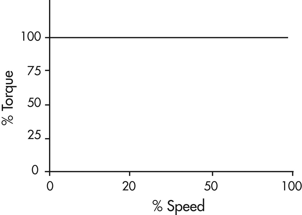
Figure 11: Constant Torque Load
Text version
Figure 11
A graph showing per cent of torque on the vertical axis and per cent of speed on the horizontal axis. There is a straight horizontal line at 100% torque representing constant torque loads from a speed range of 0 to 100%.
A constant torque load is characterized as one in which the torque is constant regardless of speed. As a result the horsepower requirement is directly proportional to the operating speed of the application and varies directly with speed. Since torque is not a function of speed, it remains constant while the horsepower and speed vary proportionately. Typical examples of constant torque applications include:
- Conveyors
- Extruders
- Mixers
- Positive displacement pumps and compressors
Some of the advantages VFDs offer in constant torque applications include precise speed control and starting and stopping with controlled acceleration/deceleration.
For constant torque loads the speed range is typically 10:1. These applications usually result in moderate energy savings at lower speeds.
Constant Horsepower Loads
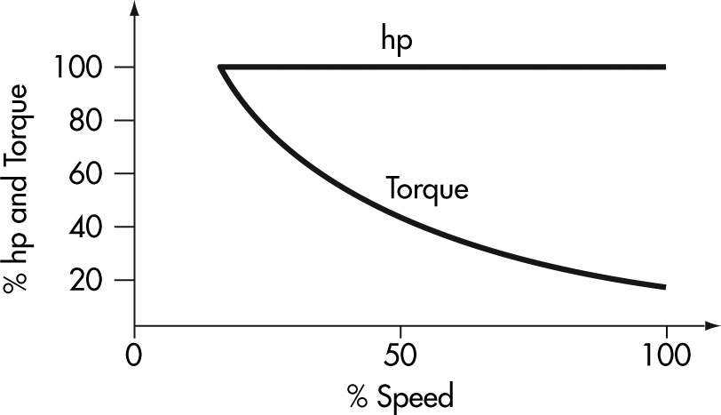
Figure 12: Constant Horsepower Load
Text version
Figure 12
A graph showing per cent of horsepower and torque on the vertical axis and per cent of speed on the horizontal axis. There is a straight horizontal line at 100% horsepower and torque representing constant horsepower loads from a speed range of 20 to 100%.
There is a second curved line representing torque beginning at 100% horsepower and torque and 20% speed and proceeding downwards to 20% horsepower and torque at 100% speed.
The second type of load characteristic is constant power. In these applications the torque requirement varies inversely with speed. As the torque increases the speed must decrease to have a constant horsepower load. The relationship can be written as:
Power = speed x torque x constant
Examples of this type of load would be a lathe or drilling and milling machines where heavy cuts are made at low speed and light cuts are made at high speed.
These applications do not offer energy savings at reduced speeds.
Variable Torque Loads
Constant Torque Loads
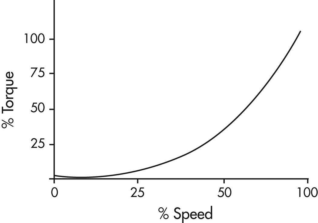
Figure 13: Variable Torque Load
Text version
Figure 13
A graph showing per cent of torque on the vertical axis and per cent of speed on the horizontal axis. There is a line curving upwards beginning at approximately 2% torque and 0% speed and ending at 100% torque and 100% speed.
The third type of load characteristic is a variable torque load. Examples include centrifugal fans, blowers and pumps. The use of a VFD with a variable torque load may return significant energy savings.
In these applications:
- Torque varies directly with speed squared
- Power varies directly with speed cubed
This means that at half speed, the horsepower required is approximately one eighth of rated maximum.
Throttling a system by using a valve or damper is an inefficient method of control because the throttling device dissipates energy which has been imparted to the fluid. A variable frequency drive simply reduces the total energy into the system when it is not needed.
- In addition to the major energy saving potential, a drive also offers the benefits of increased process control often impacting on product quality and reducing scrap.
- For variable torque loads a 3:1 speed range is typical.
Efficiencies of Motors and Drives
The full load efficiency of AC electric motors range from around 80% for the smallest motors to over 95% for motors over 100 HP. The efficiency of an electric motor drops significantly as the load is reduced below 40%. Good practice dictates that motors should be sized so that full load operation corresponds to 75% of the rated power of the motor. Figure 14 is a typical curve of motor efficiency versus loading.
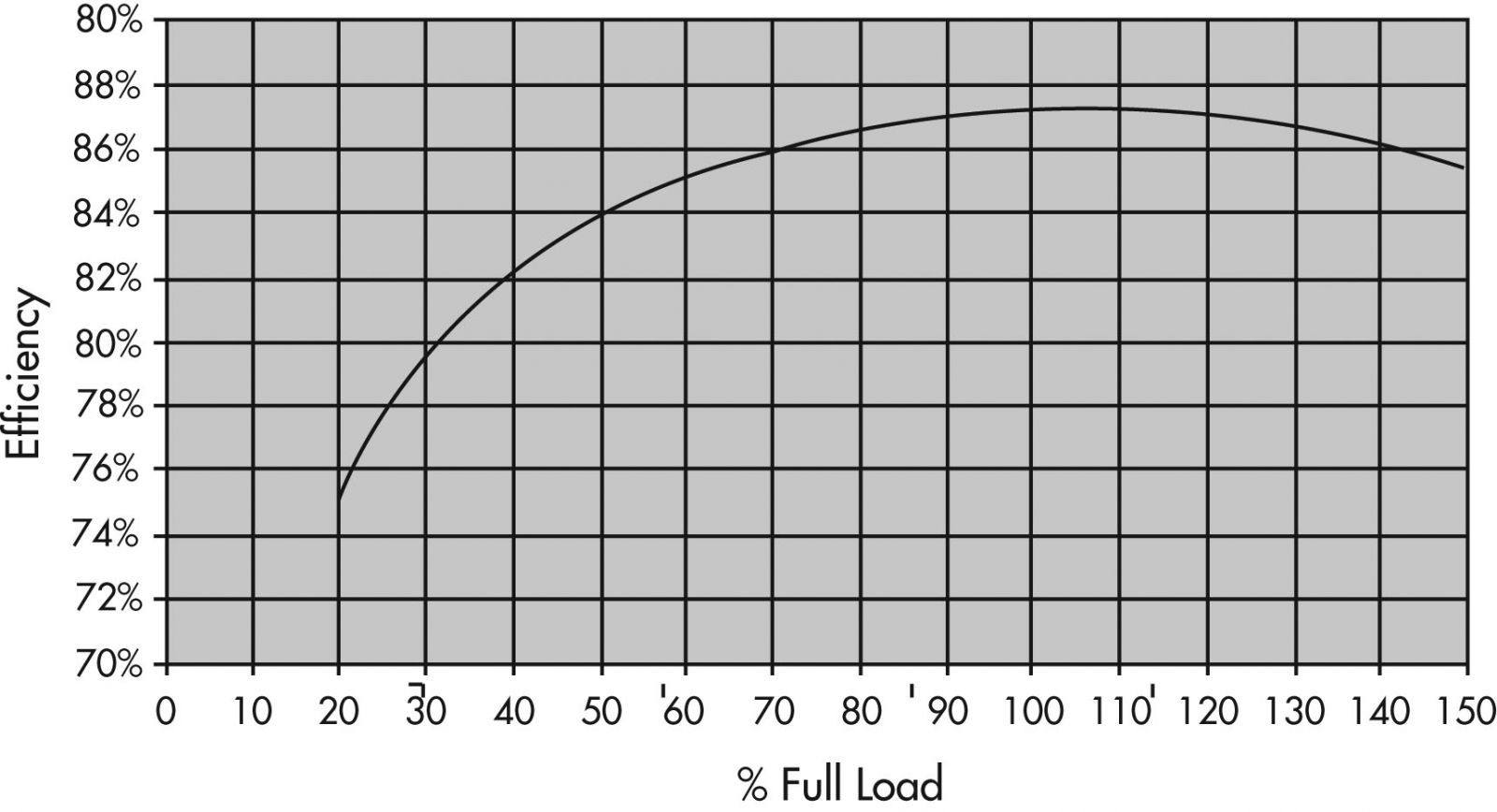
Figure 14: Typical Efficiency of a 10 HP Induction Motor Standard Efficiency Versus the Load
Text version
Figure 14
There is a second curved line representing torque beginning at 100% horsepower and torque and 20% speed and proceeding downwards to 20% horsepower and torque at 100% speed.
The efficiency of an electric motor and drive system is the ratio of mechanical output power to electrical input power and is most often expressed as a percentage.
A VFD is very efficient. Typical efficiencies of 97% or more are available at full load. At reduced loads the efficiency drops. Typically, VFDs over 10 HP have over 90% efficiency for loads greater than 25% of full load. This is the operating range of interest for practical applications.
| VFD HP rating | Efficiency % Load, Percent of Drive Rated Power Output |
||||
|---|---|---|---|---|---|
| 12.5 | 25 | 50 | 75 | 100 | |
| 1 | .48 | .74 | .84 | .87 | .89 |
| 5 | .80 | .88 | .92 | .94 | .95 |
| 10 | .83 | .90 | .94 | .95 | .96 |
| 25 | .88 | .93 | .95 | .96 | .97 |
| 50 | .86 | .92 | .95 | .96 | .96 |
| 75 | .86 | .94 | .97 | .97 | .97 |
| 100 | .89 | .94 | .96 | .96 | .97 |
| 200 | .91 | .95 | .96 | .97 | .97 |
Table from the U.S. Department of Energy’s Industrial Technologies Program – Motor Tip Sheet No. 12: Use Adjustable Speed Drive Part-Load Efficiency When Determining Energy Saving (2005 draft version).
The following table shows the efficiency of typical VFDs at various loads.
The system efficiency is lower than the product of motor efficiency and VFD efficiency because the motor efficiency varies with load and because of the effects of harmonics on the motor.
Unfortunately, it is nearly impossible to know what the motor/ drive system efficiency will be, but because the power input to a variable torque system drops so remarkably with speed, an estimate of the system efficiencies is really all that is needed.
When calculating the energy consumption of a motor drive system, estimated system efficiency in the range of 80-90 % can be used with motors ranging from 10 HP and larger and loads of 25% and greater.
In general, lower efficiency ranges correspond to small motor sizes and loads and higher efficiency ranges corresponds to larger motors and loads.
b. Comparison with Conventional Control Methods
Estimating Energy Savings
Fans and pumps are designed to be capable of meeting the maximum demand of the system in which they are installed.
However, quite often the actual demand could vary and be much less than the designed capacity. These conditions are accommodated by adding outlet dampers to fans or throttling valves to pumps.
These are effective and simple controls, but severely affect the efficiency of the system.
Using a VFD to control the fan or pump is a more efficient means of flow control than simple valves or inlet or outlet dampers. The power input to fans and pumps varies with the cube of the speed, so even seemingly small changes in speed can greatly impact the power required by the load. The table below shows the power required by a fan or pump as the speed of the machine is reduced.
| Speed of Fan/Pump | Mechanical Power Required |
|---|---|
| 100% | 100% |
| 90% | 73% |
| 75% | 42% |
| 50% | 13% |
In addition to major energy savings potential, a drive also offers built-in power factor correction, better process control and motor protection.
The most common application is the centrifugal fan or pump that imparts energy in to the working fluid by centrifugal force. This results in an increase in pressure and produces air flow at the outlet of the fan or liquid flow from a pump.
Figure 15 is an example of what a typical centrifugal fan can produce at its outlet at a given speed.
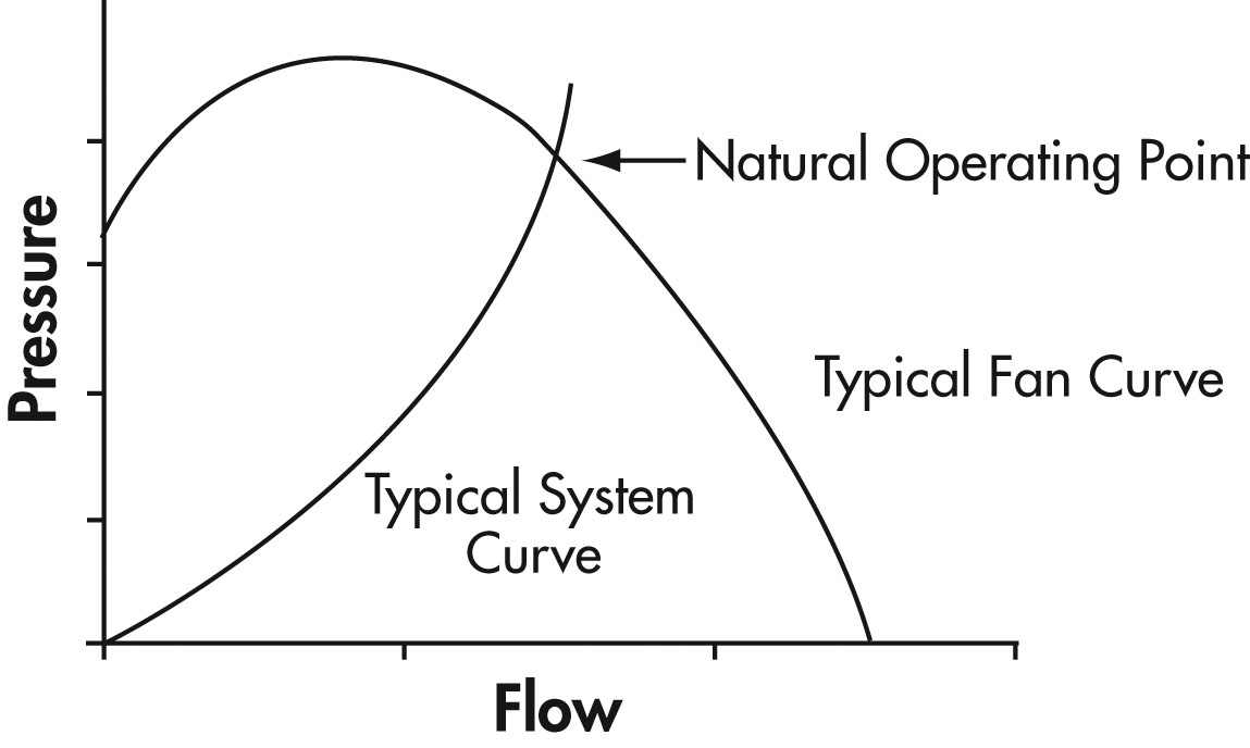
Figure 15: Plot of Outlet Pressure Versus the Flow of Air
Standard fan and pump curves will usually show a number of curves for different speeds, efficiencies and power requirements. These are all useful for selecting the optimum fan or pump for any application. They also are needed to predict operation and other parameters when the operation is changed.
Figure 15 also shows a system curve added to the fan curve. The system curve is not a product of the fan, but a curve showing the requirements of the system that the fan is used on.
It shows how much pressure is required from the fan to overcome system losses and produce an air flow.
The fan curve is a plot of fan capability independent of a system. The system curve is a plot of "load" requirement independent of the fan. The intersection of these two curves is the natural operating point. It is the actual pressure and flow that will occur at the fan outlet when this system is operated. Without external influences, the fan will operate only at this point.
Many systems however require operation at a wide variety of points. Figure 16 illustrates a profile of the typical variations in flow experienced in a typical system. How these variations are produced and controlled will have a direct effect on the energy saved.
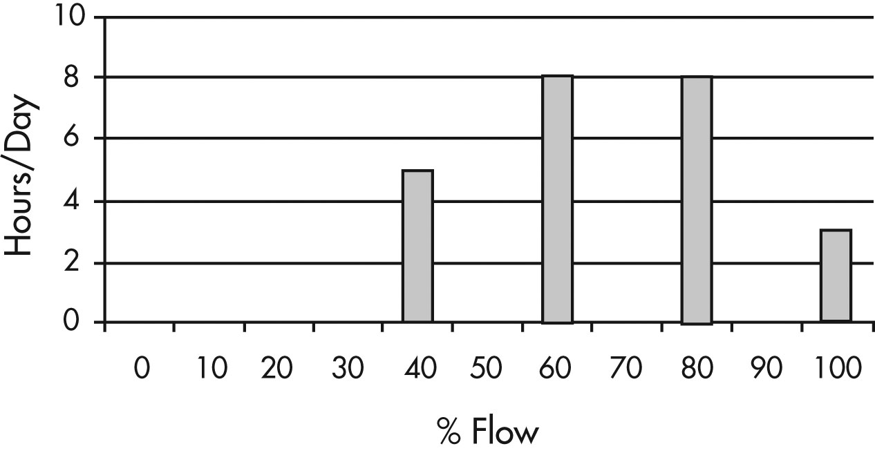
Figure 16: Variations in Flow
Text version
Figure 16
A bar chart with hours per day from 0 to 10 on the vertical axis and per cent of flow from 0 to 100 on the horizontal axis.
There are several methods used to modulate or vary the flow of a system to achieve the optimum points. Some of these include:
- Outlet dampers on fans and valves on pumps
- Inlet dampers or guide vanes on fans
- VFD control
Each of these methods affects either the system curve or the fan curve to produce a different natural operating point. In so doing, they also may change the fanâ€TMs efficiency and the power requirements.
Outlet Dampers and Valve Throttle Positions
The outlet dampers on a fan system and valves on a pump system affect the system curve by increasing the resistance to flow through their throttling action.
The system curve is a simple function that can be stated as P = K x (Flow)2. P is the pressure required to produce a given flow in the system. K is a function of the system and represents the friction to air flow. The outlet vanes affect the K portion of the formula.
Figure 17 shows several different system curves indicating different throttle positions.
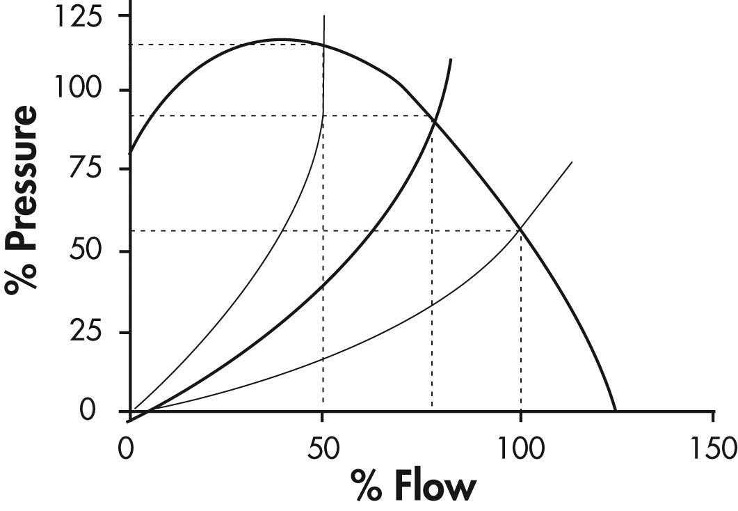
Figure 17: Pressure Versus Flow
Figure 18 presents a curve of the power requirement for this type of operation. From this curve, it can be seen that the power decreases gradually as the flow is decreased. At 50% flow 80% power is required.
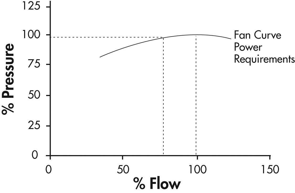
Figure 18: Pressure Versus Flow
Variable Inlet Vanes
This method modifies the fan curve so that it intersects the system curve at a different point.
There is no equivalent on a pumping system as throttling valves are never placed on the suction side of a pump.
Figure 19 illustrates several different system curves indicating different throttle positions.
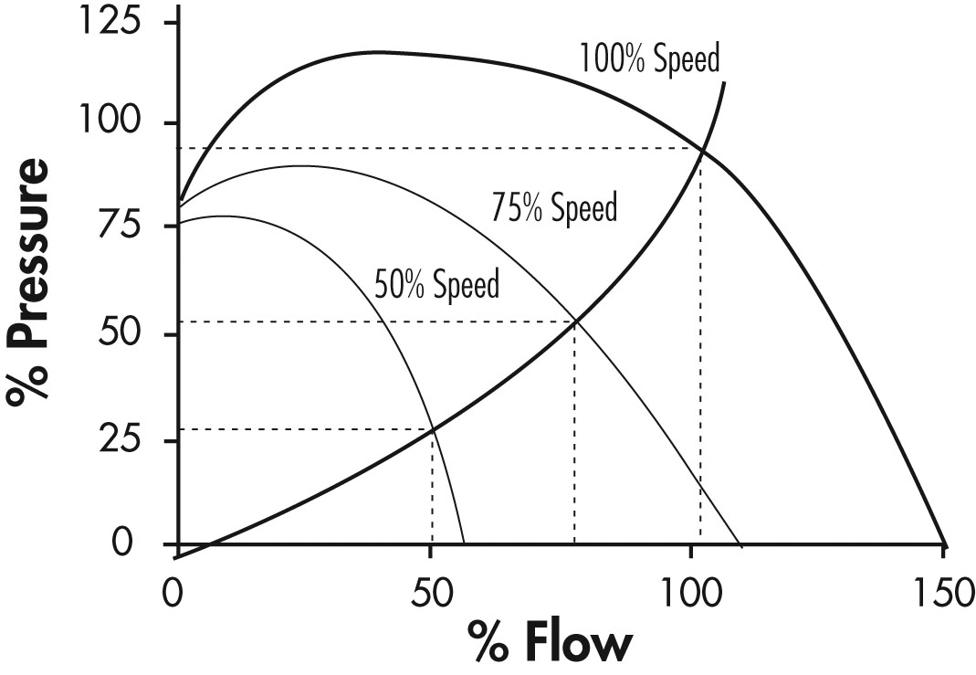
Figure 19: Fan Versus Inlet Vane Setting
Figure 20 shows that the power required by this method drops and to a greater extent than it did in the outlet throttle method. At 50% flow 60% power is required.
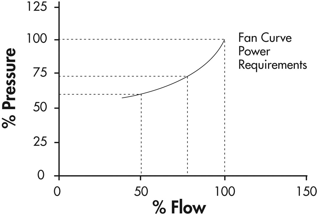
Figure 20: Fan and Inlet Vane Settings Curve
Variable Frequency Drives
This method takes advantage of the change in the fan or pump curve that occurs when the speed of the machine is changed.
These changes are quantified in a set of formulas called the affinity laws. These laws are as follows:
Where:
N = Speed
Q = Flow
P = Pressure
HP = Power
Note: when the flow and pressure laws are combined, the result is a formula that matches the system curve formula:
SYSTEM Pressure CURVE P = K x (N)².
Thus the machine will follow the system curve when its speed is changed.
Figure 21 is a representation of the adjustable-speed method.
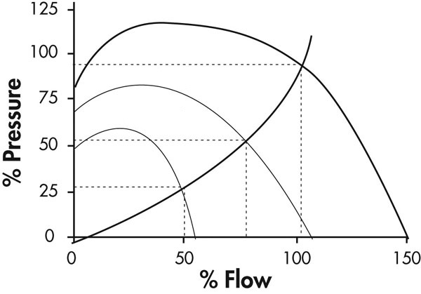
Figure 21: Adjustable-Speed Method
Figure 22 illustrates the significant reduction in power achieved by this method. The theoretical power formula from the affinity laws shows the effect of the cube functions.
Experience has shown that the actual power requirement will approximate a square function due to real life system effects like static back pressure or head, and friction so the affinity law for most real life applications is:
Where:
N = Speed
Q = Flow
P = Pressure
HP = Power
For most applications that a user will consider, the square law approximation should be used. Only fans with little or no static pressure, such as cooling tower fans and roof vent fans with domes, or pumps with no static head like discharge pumps will approximate a cube function.
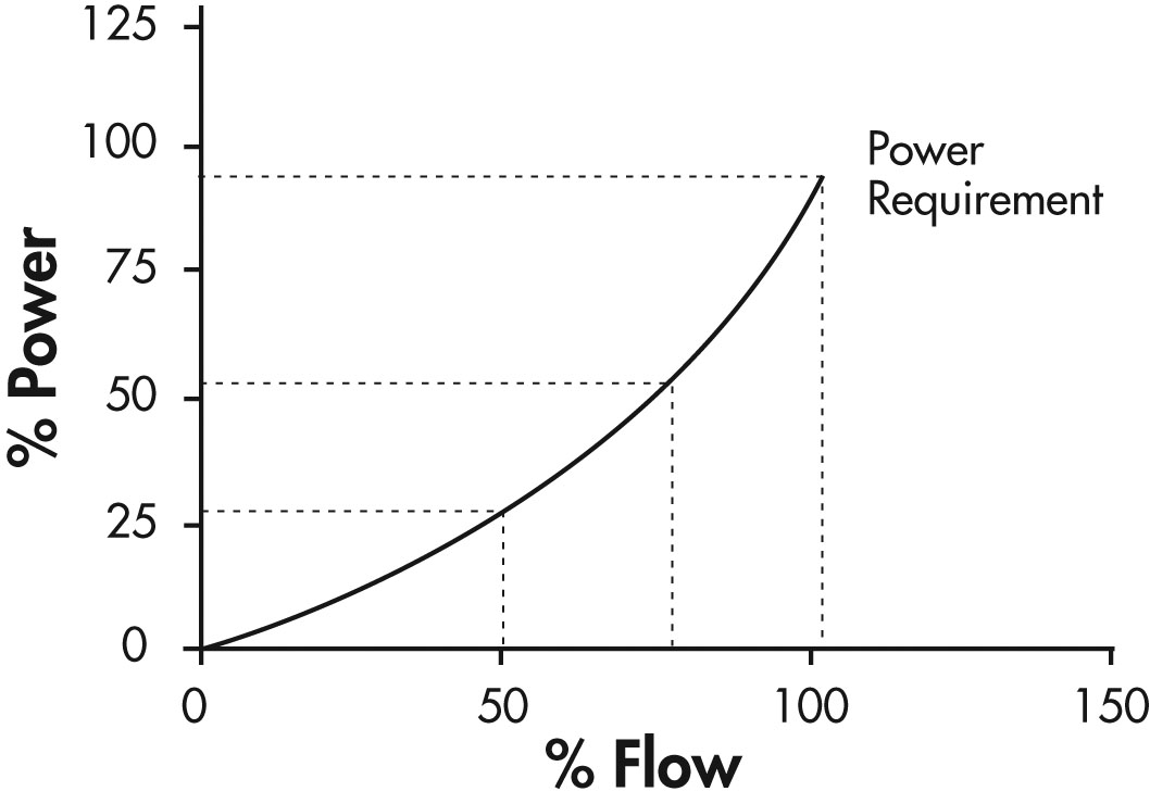
Figure 22: Square Law Approximation
Text version
Figure 22
A graph with per cent power from 0 to 125 on the vertical axis and per cent of flow from 0 to 150 on the horizontal axis.
A curve rises on the graph from 0% power and 0% flow and rises to 25% power at 50% flow, then continues to 50% power at 75% flow, and then terminates at 95% power at 100% flow.
The adjustable-speed method achieves flow control in a way that closely matches system or load curve. At 50% flow only 25% of the power is required.
This allows the fan or pump to produce the desired results with the minimum of input power.
The other two methods modify some system parameter which generally results in a reduction of the machine’s efficiency. This is why the power demand is greater than the adjustable-speed method.
Calculation of Energy Savings
It is now appropriate to estimate the power consumption and then compare the power consumption for each of the various methods to determine potential savings.
The fan selected for this example is a unit operating at 300 RPM producing a 100 percent flow rating of 2,500 m³/min, with a motor shaft power requirement of 25 kW. Pumps would be dealt with in a similar manner using the appropriate pump curve.
The fan will operate 8,000 hours per year. With no control available and at an energy cost of $0.10/kWh, the annual electricity cost will be:
(25 kW) (8,000 hrs) ($0.10/kWhr) = $20,000 /year
To determine the potential savings from a control method, a load profile must be developed. For this example, the following load profile is determined:
| Flow | Duty Cycle |
|---|---|
| 100% | 20% |
| 75% | 40% |
| 50% | 40% |
Required Power
For each operating point, a required power from the fan curve can be obtained (from the preceding curves for each control scheme).
This power is multiplied by the percent of time that the fan operates at this point. These calculations are then summed to produce a “weighted power” that represents the average energy consumption of the fan.
From the outlet damper curve (Figure 18), the weighted power calculations for the outlet damper method are as follows:
| % Flow | % Duty Cycle | Power Required (kW) | Weighted Power (kW) |
|---|---|---|---|
| 100 | 20 | 25 (1.00) = 25.0 | 25.0 (0.2) = 5.0 |
| 75 | 40 | 25 (0.96) = 24.0 | 24.0 (0.4) = 9.6 |
| 50 | 40 | 25 (0.88) = 22.0 | 22.0 (0.4) = 8.8 |
| Average Annual Power | 23.4 kW | ||
The weighted power calculations for the variable inlet vane (Figure 20) method are as follows:
| % Flow | % Duty Cycle | Power Required (kW) | Weighted Power (kW) |
|---|---|---|---|
| 100 | 20 | 25 (1.00) = 25.0 | 25.0 (0.2) = 5.0 |
| 75 | 40 | 25 (0.73) = 18.3 | 18.3 (0.4) = 9.6 |
| 50 | 40 | 25 (0.60) = 15.0 | 15.0 (0.4) = 6.0 |
| Average Annual Power | 20.6 kW | ||
The weighted power calculations for the VFD (Figure 22) method are as follows:
| % Flow | % Duty Cycle | Power Required (kW) | Weighted Power (kW) |
|---|---|---|---|
| 100 | 20 | 25 (1.00) = 25.0 | 25.0 (0.2) = 5.0 |
| 75 | 40 | 25 (0.55) = 13.8 | 18.3 (0.4) = 5.5 |
| 50 | 40 | 25 (0.25) = 6.3 | 15.0 (0.4) = 2.5 |
| Average Annual Power | 13.0 kW | ||
The annual cost of operation for the three control methods are as follows:
Outlet Dampers : 23.4 kW x $0.10/kWhr x 8000 Hours x $18,720
Inlet Dampers : 20.6 kW x $0.10/kWhr x 8000 Hours x $16,480
VFD Control : 13.0 kW x $0.10/kWhr x 8000 Hours x $10,400
The savings from these control methods are as follows:
| Control Type | Annual Operating Cost | Annual Savings |
|---|---|---|
| None | $20,000 | 0 |
| Outlet Dampers | $18,720 | $1,280 |
| Inlet Dampers | $16,480 | $3,520 |
| VFD Control | $10,400 | $9,600 |
The above calculations use a simple “blended” cost for electricity. How your utility charges for electricity usually depends on a number of factors including demand, energy, time of use and other factors. Your local utility representative should be contacted for more detail on how to calculate your electricity cost.
VFD Savings Software
Software is available from several VFD manufacturers, suppliers and in some cases local utilities along with government organizations.
These resources are very useful for estimating energy savings and exploring control options. Several will allow performance data to be input when it is available to make the analysis even more accurate.
Each source of software assumes a basic understanding of VFD technology and a thorough understanding of the application.
c. Monitoring and Verification
It is important to establish a Measurement and Verification plan (M&V) ahead of the project execution for several reasons, including:
- Proving the estimated savings is achieved.
- Meeting conservation and demand management incentive application requirements.
- Obtaining support for future projects through demonstrating success.
Energy savings are determined by comparing the energy use before the project starts (base case) and then again after the installation of the energy conservation measures (post project).
Proper determination of savings includes adjusting for changes that affect energy use but that are not caused by the conservation measures. Adjustments will vary on the application and include considerations such as weather, product or occupancy conditions between the baseline and post installation periods.
M&V activities generally take place in the following steps:
- Define the pre-installation baseline, including:
- equipment and systems
- baseline energy use (and cost)
- factors that influence baseline energy use.
- Define the post-project installation situation, including:
- equipment and systems
- post-installation energy use (and cost)
- factors that influence post installation energy use.
- Site surveys, spot, short-term, or long-term metering, and/or analysis of billing data can be used for the post-installation assessment.
- Conduct ongoing M&V activities to verify the operation of the installed equipment/systems, determine current year savings, and estimate savings for subsequent years.
Note: Adding a VFD is often part of an equipment upgrade.
This can affect process flow or related operations. It is important that the post project energy use is equally adjusted to match the pre-installation operating conditions.
Measurement and verification can be a fairly complex process and the success of the current VFD project or future energy efficiency projects may depend upon an accurate and detailed measurement and verification process. It must be included as part of the project costs. It is recommended that a professional practitioner be used to ensure that the measurements are done correctly. Usually the costs associated with the M & V can be recovered from available incentives.
The CEATI Energy Savings Measurement Guide provides details on the process for undertaking measurement and verification of the project.
d. System Efficiency
System efficiency is defined as the ratio of the units of product produced by that system to the electrical energy drawn by a system. To determine any difference, subtract the old system efficiency from the new.
If the number is negative, then the system efficiency has declined since the system optimization. The outcome should always be positive.
e. Electrical Efficiency
The electrical efficiency improvement is determined by comparing the base case measured electrical consumption with the electrical use determined during the project evaluation metering.
Efficiency Improvement = Post Project Efficiency – Base Case Efficiency
f. Cost Per Unit Product
This calculation incorporates billing data to give a dollar value to the optimization. Using the formula presented in the base case, apply the post-project metering data.
[Demand Charge for Motor + (OP kWh * OP Rate + FP kWh x FP Rate)]
Divided by:
# of Units Produced per Day
OP Rate = the rate per kWh of on-peak energy consumption
FP Rate = the rate per kWh off off-peak energy consumption
To compare against the base case, subtract the base case number from the post-optimization number. If the resulting number is negative, then the cost per unit product has increased. The number should always be positive.
g. Reliability and Maintenance
Solid-state electronics in VFDs are relatively maintenance free.
Most drive manufacturers supply built-in diagnostics as well as protection relays and fuses.
When service is required, trained personnel are needed to troubleshoot and repair the drive.
Routine maintenance may include cleaning/replacing filters where fitted in addition to standard electrical maintenance activities such as cleaning and inspection on a regular basis.
When repairing electric motors being operated by VFDs, the repair shop should utilize "inverter duty" magnet wire in any rewinds. In addition, they should not reduce the number of turns in coil groups as this increases the electrical stress per turn in the winding.
If the motor failed due to overheating, consideration should be given as to whether sufficient cooling is available to the motor. Fitting an external cooling fan or over-sizing the motor are two options that may be considered.
Your drive supplier or motor repair shop will be able to provide assistance for any service problems.
Page details
- Date modified: