
ARCHIVED - Energy Efficiency in Buildings
Information Archived on the Web
Information identified as archived on the Web is for reference, research or recordkeeping purposes. It has not been altered or updated after the date of archiving. Web pages that are archived on the Web are not subject to the Government of Canada Web Standards. As per the Communications Policy of the Government of Canada, you can request alternate formats. Please "contact us" to request a format other than those available.
Benchmarking Guide for School Facility Managers
Table of Contents
Section 1. Energy Use in Schools 1
Section 2. Benchmarking Energy Performance
Section 3. The Benchmark Results
Section 4. Step-by-Step Sample Benchmark Comparisons
Section 5. Calculating Greenhouse Gas (GHG) Emissions
Section 6. Conversion Factors, Energy Contents, GHG Emission Factors and Heating Degree-Days (HDD)
Introduction
The Benchmarking Guide for School Facility Managers is intended to help facility managers in the school sector calculate their schools' energy performance and compare it with benchmarks in the same region and across Canada. The objectives of the guide are to be an "eye opener" and to raise questions. Benchmarking can help facility managers gauge their schools' energy performance to identify opportunities for cost savings. By comparing their buildings' average intensities with other schools at the national and regional levels and with similar schools, facility managers can set targets for improved performance. Identifying and following through on opportunities to reduce energy consumption can save money and improve the environment.
This benchmarking guide is published in conjunction with the Best Practices Guide for School Facility Managers. The guides are part of the pilot benchmarking and best practices program undertaken by Natural Resources Canada's (NRCan's) Office of Energy Efficiency (OEE).
Section 1. Energy Use in Schools
Getting started involves finding out where energy is being used and determining the main areas that can be improved. In schools, energy is used to provide a comfortable and safe environment for educational, sporting and administrative activities, and for additional facilities (such as catering, laboratory equipment, swimming pools and gymnasiums). Heating and lighting are the main services but, depending on location, the school may also have some mechanical cooling or air-conditioning requirements. Heating is generally by a gas- or an oil-fired boiler. Some direct electric heating is also used where low-cost, renewable, electricity supplies are available (e.g. some areas of Quebec and almost all rural schools in Manitoba are electrically driven). Mechanical cooling is driven by electricity.
Fossil fuel for heating may be the largest element of the site's energy use and hence appears to be the largest on-site source of carbon dioxide (CO2) emissions. However, when primary energy use (including power station conversion) is calculated, air conditioning can produce the largest amount of CO2 and can be a major cost. Keeping track of both systems should be a major objective of any comprehensive energy monitoring and tracking program. In schools with special equipment and facilities (e.g. swimming pools), energy costs and consumption should be separately monitored and tracked to keep costs within budgets.
1.1 Energy Consumption in Canadian Schools
There are approximately 15 000 schools in Canada administered by about 495 school boards. Energy consumption data have been analysed to prepare this benchmarking guide. Figure 1 and Table 1 show the energy use and costs data that were gathered during this first pilot program. About 1473 schools responded to the OEE's data collection process. The Agence de l'efficacité énergétique and Quebec's Ministère de l'Éducation provided additional data from 2770 schools in Quebec (see Section 7, Resources). Because fiscal years vary, the data are based on 1997-1999.
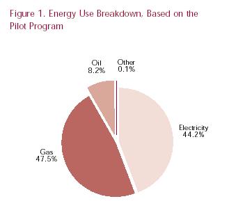
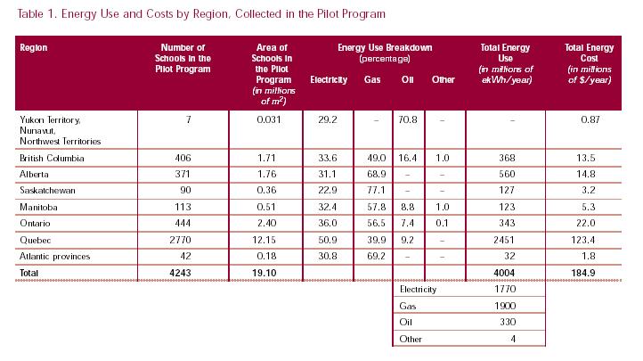
Notes:
- ekWh/year = equivalent kilowatt hours delivered energy per year.
- The "Other" category of Energy Use Breakdown includes liquefied petroleum gas (LPG) and solid fuels.
- Table 1 is not to be used for comparison purposes. School boards may not have provided complete information. Some school boards provided either energy consumption or costs, not necessarily both. Therefore, $/ekWh for each region may be significantly different.
- The data are based on the period 1997-1999.
Section 2. Benchmarking Energy Performance
Information on energy performance provides the basis for monitoring and tracking energy use. Regular collection of basic data can help evaluate performance and pinpoint potential savings. Patterns or trends in fuel use can be identified by benchmarking data against similar schools, regionally and nationally, and by comparing results on a yearly basis.
Benchmarks provide representative data. A school can compare its performance with national figures of annual energy use, or costs per square metre of floor area or per student. This way, school facility managers can see the potential benefits of achieving "best practice."
Performance can vary from the benchmarks, depending on impact variables (or influencing factors). A limited amount of data was obtained in this pilot program, so some impact variables were not considered. Influencing factors considered in this Guide include the following:
- Location - Benchmark data are expressed by geographic region. Location can affect energy performance because different regions may use different sources of energy or have different rates for energy costs.
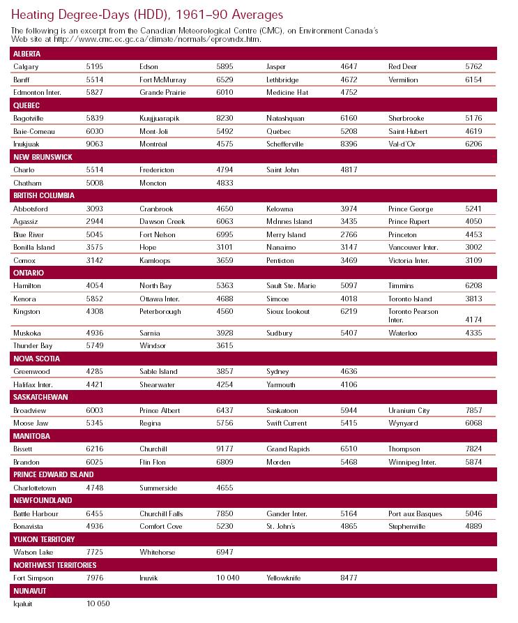
- Climate - Each location has heating and cooling degree-days. They reflect the total number of degrees for equivalent days in a given period for which heating and/or cooling are needed to achieve standard indoor conditions at a specified location. They provide a basis for comparing different climatic regions in terms of energy use per heating and/or cooling degree-days. Heating degree-day (HDD) measures the amount of heating energy required during the heating season; it is measured by the difference between the base temperature of 18oC and the mean temperature for the day.
To account for HDD, energy consumption was normalized using the methodology provided by the Agence de l'efficacité énergétique and Quebec's Ministère de l'Éducation. The average HDDfor the past 30 years and for the specific year were obtained from Environment Canada to normalize the data (see Section 7 for references). Following is the formula used to normalize for HDD:
En = Ea × [0.3 + 0.7 (HDD30/HDDa)]
Where,
En = normalized annual consumption for a year
Ea = actual annual consumption for a year
HDD30 = 30-year annual average heating
degree-days (based on 18oC)
HDDa = actual annual average heating degree-days
(based on 18oC)
- Occupancy - Intensity data are based on equivalent student numbers, which include full- and part-time students. The equivalent number of students is important in schools that offer night classes or curricula at other times because part-time students are an indicator of longer operating hours. Occupancy is one way to account for the impact of these hours.
- Building age - Benchmark data are available for sites with buildings in three age categories: more than 25 years, 10 to 25 years, and less than 10 years.
In addition to impact variables, this Guide includes benchmarks for various levels within the school board sector. Facility managers can compare energy performance with other school boards, within their own school board, or with similar schools in other school boards. This may help determine whether to pursue energy efficiency actions as a school board or within an individual school. Levels within the sector include the following:
- School boards - Energy consumption intensities of school boards can be compared to national and regional averages. Similarly, cost intensities are provided as an example. The impact variables considered are energy consumption and costs, HDD, floor area, number of students and geographic region.
- Individual schools - Energy consumption intensities for individual schools can also be compared to national and regional averages. Likewise, the variables considered for individual schools are energy consumption and costs, HDD, area, students and geographic region. Originally, individual schools were placed into categories: elementary, high school and other. But the results did not show significant differences. Therefore, in this Guide the three types of schools are grouped as a single school.
- Similar schools - The third level of benchmarking is comparison with similar schools. A school can be compared with schools that have similar HDD and building age, as well as whether they use air conditioning or not.
The results of the first pilot national survey of benchmark performance are shown in Section 3.
2.1 Calculating the Benchmarks
Calculating your school board's energy benchmark involves collecting data on occupancy, annual energy use, climatic variations and physical characteristics of the site. The following sections describe the procedures for benchmarking a school board's energy consumption and cost intensities.
2.1.1 School Board Benchmark Performance
To calculate your school board's benchmark and to compare it with the data in this Guide, follow these steps:
-
Collect information on the total floor area(s) in square metres (m2) that is/are serviced - i.e. heated and/or cooled.
-
Determine the total number of students in the school board.
-
Collate meter readings or utility bills to derive the annual costs and energy consumption of fossil fuel and electricity for all the schools in the school board.
-
Convert consumption data to common energy units -equivalent kilowatt-hours (ekWh) - and derive the total consumption. (See Section 6 for information on conversion factors and where you can obtain extra help for conversions.)
-
Obtain the average annual HDD for the past 30 years and annual HDD data for the specific year for your region.
-
Normalize the energy consumption for HDD, using the equation provided on page 3.
-
Calculate the overall benchmark performances for the actual and normalized energy intensities - in ekWh/m2, ekWh/student, $/m2, $/student. Then compare your results with the benchmark data in Figures 4 and 5 and Tables 2 and 3 (found in Section 3).
This gives you the overall benchmark performance for your school board. A template to help you calculate the benchmarks is provided in Figure 2.
Costs and student comparisons are provided only to give an indication. As you will see in the benchmark results in Section 3, costs and student comparisons show significant variations due to many factors, including differences in unit cost of energy.

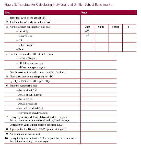
2.1.2 Individual School Benchmark Performance
You can compare individual schools by following an almost identical method to the one that you used for school boards (discussed above). Follow all of the steps for school boards, using Figure 3 as a template to gather the necessary information and make the appropriate calculations.
Once again, use costs and student comparisons only as examples of benchmarks. (Student comparisons may vary due to several different factors, some of which were previously mentioned.)
2.1.3 Similar School Benchmark Performance
The third level of benchmarking in this guide is comparison with similar schools. The impact variables considered are climate (HDD), age of school, location of school and air conditioning.
Figure 3 can also be used to summarize the data in order to compare your findings to the benchmark results in Section 3.
2.2 Comparison with the Model National Energy Code for Buildings and the Commercial Building Incentive Program (CBIP)
Another useful type of benchmarking that schools can undertake is comparison with the requirements of the Model National Energy Code for Buildings (MNECB) and the Commercial Building Incentive Program (CBIP). Although not in the scope of this benchmarking program, this type of comparison is noteworthy.
The OEE uses the MNECB as the basis for comparison under CBIP. The MNECB sets minimum standards for building components and features that affect energy efficiency in buildings. One main CBIP requirement is that a building's energy use be at least 25 percent lower than that of a similar structure built to the MNECB's standards. The MNECB helps designers introduce energy-efficient buildings that minimize air-conditioning and heating bills. It considers climate, fuel types and costs, and regional construction costs to calculate minimum standards. The MNECB also addresses thermal resistance; lighting efficiency; heating, ventilating and air conditioning (HVAC); service water use; and general electrical consumption.
Energy-using buildings and equipment in schools are generally designed according to the standards of performance set by the American Society of Heating, Refrigeration and Air-Conditioning Engineers (ASHRAE). Facility managers can refer to ASHRAE codes for further advice on energy performance and the design of improvement measures. For more information on how to compare your facilities with CBIP's requirements, see Section 7, Resources.
Section 3. The Benchmark Results
In this pilot benchmarking pilot program, 1997-1999 data from 112 school boards and 4243 schools have been analysed to derive national and regional patterns. Because the amount of data is limited, the benchmarking approach described below was taken.
The patterns are illustrated in various x-y (scatter) graphs and summarized tables. A graphical representation of the data is provided using trend lines. These trend lines were analysed using a statistical technique called regression analysis. R-squared (R2) values, or the proportion of the variance in y caused by the variance in x, are also provided. They show if there is a relationship among the various impact variables, such as area, HDD and students. The closer the value (or R2) is to 1, the stronger the relationship.
The basic data in this Guide are presented without attribution (which is normal for such an exercise). The following analysis is based on a limited sample of data from school boards that responded to a questionnaire conducted by the OEE, or obtained from the Agence de l'efficacité énergétique and Quebec's Ministère de l'Éducation. In some cases, the data were incomplete and/or only historic information was available. There was also a significant discrepancy among regions related to the level of coverage. Therefore, the results should be regarded as a preliminary view of benchmark performance for the Canadian school sector.
An indication of savings may stimulate further detailed analysis on-site. Standards will steadily improve as further measures are implemented. The level of "good" and "best practice" performance should be lower in subsequent surveys.
Schools can use this benchmark data to determine how their energy performance compares. Schools with energy performance at or below the average - either below the regression line or the average equation (i.e. ekWh/m2) - could be showing "good practice." Those with performance 25 percent or more below average could fall under the "best practice" category.
By using trend lines, schools can calculate "average" performance for their site or student numbers and then compare it with their current energy use.
The difference between "good" and "best" practice gives a global indication of potential savings for the site.
3.1 School Board Energy Performance
Data from school boards that submitted enough information were analysed to determine the relationships among different impact variables, including the following:
- climate (HDD);
- region;
- energy consumption and cost;
- floor area; and
- number of students.
These variables were used on a national level and by each geographic region. Thus the following benchmarks for the school boards were set (using x-y graphs):
- ekWh vs. area (m2) for both actual and normalized annual energy consumption;
- ekWh vs. number of students for both actual and normalized annual energy consumption;
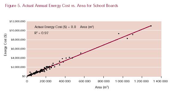
- actual annual energy costs ($) vs. area (m2); and
- actual annual energy costs ($) vs. number of students.
Note: All information is based on annual data.
The following figures and table show the results of the benchmark analysis.
Note:
- The cost benchmarks are provided only as an illustration and, therefore, should be used with caution. Unit costs from region to region and from school board to school board can vary significantly, which can dramatically influence the cost benchmarks.
Results and Observations
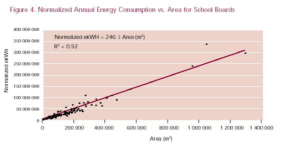
The data from school boards were used to determine the average consumption and cost intensities for use as reference points. The data were normalized to take HDD into account. For each school board, consumption and costs were plotted against area and number of students to determine whether a relationship existed. Figures 4 and 5 and Tables 2 and 3 represent the energy intensity results for consumption and costs. It is clear from the regressional analysis that a correlation exists between consumption and area or students.
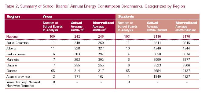
Normalized and actual intensities - The difference between the national normalized ekWh/m2 and actual ekWh/m2 was almost 2 percent. However, the difference in some provinces was higher; British Columbia's normalized intensity was 8.3 percent higher than the actual. Clearly, climate impacts energy performance.
ekWh/m2- Area had a strong relationship with consumption, with a national R2 value of 0.92. The lowest correlation was for Manitoba, which had an R2 value of 0.85. The Prairie provinces appeared to consume more energy per square metre than other provinces, especially Quebec and British Columbia. The Prairie provinces also seemed to consume more than the national average. However, since Quebec was heavily represented in the survey and had the lowest consumption per square metre, it may be skewing the national average. It is interesting to note that as school board size increases, intensities show greater variation. Therefore, school boards with smaller areas tend to consume similar amounts of energy per square metre.
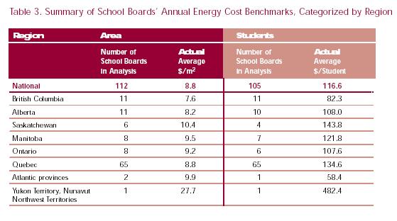
$/m2 - Cost also seemed to be affected by the size of the school board, with a national R2 value of 0.97 indicating a very strong relationship. All provinces incurred similar costs per square metre, which is somewhat surprising since these costs should vary among regions. Based on the normalized cost performances, Saskatchewan paid slightly more (about 18 percent) per square metre than the national average. British Columbia had the lowest cost intensity. The territories had by far the highest cost per square metre, but this could be due to their low survey response rate. What is surprising is the trend for the cost per square metre to increase as the area of the school board increases.
ekWh/student - A correlation between consumption and students, although less obvious, also existed. Except for Saskatchewan, all R2 values were over 0.75. School boards with more than 15 000 students seemed to have more variations in energy intensities. As the number of students increased in a school board, the relationship between consumption and students weakened. Provincial averages varied significantly. This may suggest that the methodology used for reporting the number of students varied from province to province. The Atlantic provinces had a notably lower average, which is likely due to their low survey response rate.
$/student - Although somewhat surprising, a fairly strong relationship existed between cost of energy and students, which does not account for regional differences in unit prices for different school boards. R2 values were greater than 0.6. Similar to the consumption-per-student results, the cost per student increased as the number of students within the school board increased. The average costs per student did vary from region to region, with the British Columbia average about 29 percent lower than the national average and the Saskatchewan average 23 percent higher. The territories and the Atlantic provinces had drastically lower averages, but fewer school boards responded to the survey.
3.2 Individual School Energy Performance
Relevant data were collected for individual schools in an effort to determine benchmark performance for each school. Data from about 3500 schools were used to determine the relationships among different impact variables and to set relevant benchmarks. The approach taken to benchmark school energy performance was similar to that for school boards. The following figures and tables provide the benchmark results.
Results and Observations
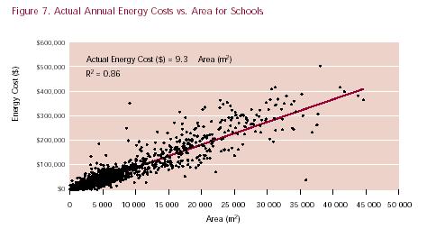
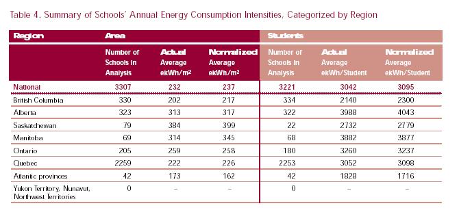
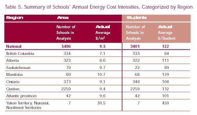
Like the school boards, energy consumption and costs for individual schools were plotted against area and number of students to determine whether a relationship existed. The benchmark results are depicted in Figures 6 and 7 and Tables 4 and 5.
Normalized and actual intensities - The difference between the national normalized ekWh/m2 and actual ekWh/m2 was about 2 percent. However, the difference in some provinces was higher, with British Columbia's normalized intensity being 7.4 percent higher than its actual intensity.
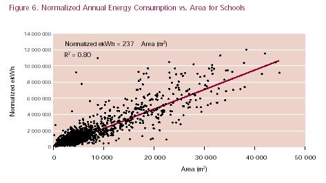
ekWh/m2- With an R2 value of 0.8, a significant relationship existed between consumption and area for schools. Regardless of size, the energy intensities for individual schools varied significantly. The performances for Alberta, Saskatchewan and Manitoba were noticeably above the national average. Quebec, British Columbia and the Atlantic provinces had the lowest averages, which could indicate that the schools in these regions were more energy efficient than those in other regions. However, the low average in the Atlantic provinces could be attributed to the low number of data points; in British Columbia, the R2 value was 0.48, which suggests a lower degree of correlation between energy and area. The variance was greater for schools larger than 8500 m2, as seen in Figure 6. In some cases, several schools with an area of 8500 m2 had performances much lower than the average. This may suggest that these schools are considerably more efficient than the others; perhaps they have implemented a "best practices" program. However, in other cases, numerous schools had averages that were much higher than the national average. This may be due to either inefficient practices or uncommon services such as swimming pools.
$/m2 - Energy costs had a stronger relationship with area, with an R2 of 0.86 for the national cost performance. Although weak in some provinces, such as British Columbia (R2 = 0.58) and Ontario (R2 = 0.64), the relationship was high enough to conclude that area is an impact variable. Some degree of variance existed among the costs in different provinces. The territories, Saskatchewan and Manitoba had the highest cost per square metre, while British Columbia had the lowest. The variations were expected, as different regions have different rates for energy consumption. Only the territories had a drastically different average from the national average. The cost per square metre for the territories was much higher than in other regions. But this would not affect the national average because there was a minimal number of schools from the territories in the analysis. The relationship between cost and area (R2 = 0.86) for national intensity was slightly higher than for consumption and area (R2 = 0.80), which could suggest that there is a more consistent unit of cost - compared to consumption -across Canada per square metre.
ekWh/student and $/student - A weak relationship also existed between consumption and costs, and size of school. Because the national R2 values for consumption and costs were 0.9 and 0.6 respectively, it can be concluded that students can also be an impact variable. However, a great degree of variance exists among the provinces. The consumption relationship was the weakest in Saskatchewan, which had an R2 value of 0.36. The relationship was significantly stronger in other regions, with one R2 value as high as 0.95. As for the impact of students on costs, there were greater variations in R2 values for each province. Most of the R2 values were below 0.65. This may suggest that either the impact of students on costs is less or different methods determine student counts.
3.3 Similar School Energy Performance
To help schools compare their performance with other sites with similar characteristics, the national survey data were analysed further. It considered the effects of other variables - including climate, type of operations at the schools, and number and age of buildings - to determine which variables influenced energy use significantly.
It should be noted that original research included more variables related to grouping similar schools. However, due to the lack of data, no concise conclusions could be made. Therefore, many impact variables were either ignored or mentioned as sub-variables (see Section 3.4).
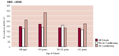
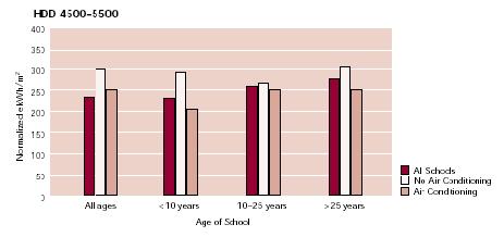
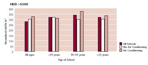
Based on the data collected, three variables were considered for comparing energy performances with similar schools: HDD, age of school and the presence/use of air conditioning in the school. The type of school (e.g. elementary or secondary) was not considered because the national energy intensities did not show significant deviation (as shown in the previous section).
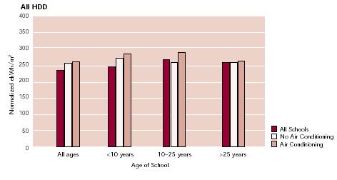
The results are presented in the next four graphs. The age of the schools is broken into four categories:
- all ages (which includes data - regardless of age - from all schools, including those in Quebec);
- ages less than 10 years;
- ages from 10 to 25 years; and
- ages greater than 25 years.
The data from Quebec were not considered to calculate the averages for the individual age groups. For each HDD range and age of school category, the average performances are presented for
- all schools, whether they have air conditioning or not;
- schools with air conditioning; and
- schools without air conditioning.
Notes:
- "All Schools" includes schools that did not identify whether they operated air-conditioning units and includes data from Quebec.
- The data from Quebec are excluded from the age sub-group analysis.
Results and Observations
A comprehensive analysis was not possible with the limited amount of data on certain variables. Therefore, the following conclusions should be regarded only as examples. The previous graphs show the results of the energy intensity performances for the various groups that are considered similar schools.
Despite the limited data, some preliminary observations were made, including the following:
- As HDD increased, the average energy intensities (ekWh/m2) increased from 195 for HDD >4500 to 270 for HDD >5500. This may suggest that cooler regions require more heating, which would increase consumption.
- The highest intensity of 374 ekWh/m2 was yielded in the 10-25 years age group for HDD >5500.
- Clearly, schools with air conditioning consumed higher energy than those without, except in the case of HDD from 4500 to 5500. The intensities of schools with air conditioning were from 1.5 percent to 43 percent higher than those without air conditioning. The few cases where the intensities of schools with air conditioning is lower may suggest that these schools are more efficient.
- For all HDD groups, the normalized intensity was highest in the 10-25 age category. This may suggest that older schools (>25 years) may have been retrofitted as a result of aging equipment and systems. By doing this, the schools could have increased their energy efficiency.
3.4 Other Impact Variables Considered
As part of the analysis, several other impact variables were considered, including use of air conditioning, central ventilation, portable buildings and operating hours. Due to the lack of data, the impact variables were not included in the comparison with similar schools.
Computers
Over the past 10 years, computer use in schools has dramatically increased. This has resulted in an increase in energy consumption and costs. The number of computers at a school can range from 10 to 100. Each computer can consume 29-120 W and cost between $10 and $30 per year. Therefore, computer use can increase a school's consumption and costs by 5 percent.
Air Conditioning
The use of air conditioning varied in schools across Canada. Most new schools operated central air-conditioning systems. On the other hand, the majority of the older schools did not have air conditioning. From the data, it is estimated that an average school with an air-conditioning system can consume 15 percent or 10-40 kWh/m2 more energy than those without. It can cost the school $1.30-$2.50/m2 to operate these units.
Central Ventilation
Most schools had some form of ventilation system. However, while most new schools had central ventilation systems, many of the older schools did not. It was shown that central ventilation could increase energy use by up to 30 percent or 20 kWh/m2.
Portable Buildings
Portable classrooms can have lower thermal efficiency than permanent structures and need more heating energy. Low thermal mass can also increase heat gains in summer, making air conditioning necessary. Energy consumption per unit area, particularly electricity, may be up to 20 percent greater for sites with portable buildings. Heating systems with rooftop-mounted gas-fired units or direct electricity and cooling by direct expansion units have basic controls only. In such buildings, actual use should be identified and a careful monitoring and tracking system instituted. Controllers that can be programmed for heating and/or cooling systems may be a worthwhile investment.
Swimming Pools
Finally, the impact of swimming pools in the schools' energy consumption was also considered. A marginal number of schools had swimming pools, so the benchmark comparison for similar schools was not sorted into those with pools and those without. Instead, the impact of pools was analysed. Based on the limited number of data, it is suggested that schools with swimming pools could consume 15-25 percent more energy than those without pools.
3.5 Comparison with Commercial Building Incentive Program (CBIP) Requirements
Schools can use the CBIP requirements to benchmark their existing energy performance against reference examples for their region. As mentioned in Section 2.2, one key CBIP requirement is that a building's energy use must be at least 25 percent lower than that of a similar structure built to the MNECB's standards. This amount of energy use should provide an overall level of savings potential. For more information on the procedures for benchmarking against CBIP requirements, see the contact details in Section 7.
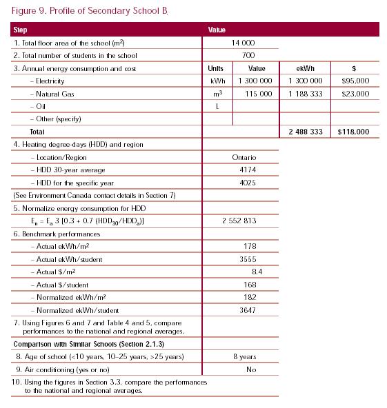
Section 4. Step-by-Step Sample Benchmark Comparisons
The following section is a step-by-step example showing how to use this guide to compare average intensities for a sample school board (School Board A) and an individual school (Secondary School B). Their characteristics are summarized in Figures 8 and 9, which use the templates from Figures 2 and 3. Observations are provided to give the type of analysis and the conclusions that can be made as a result of the comparison.
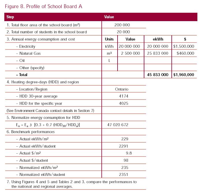
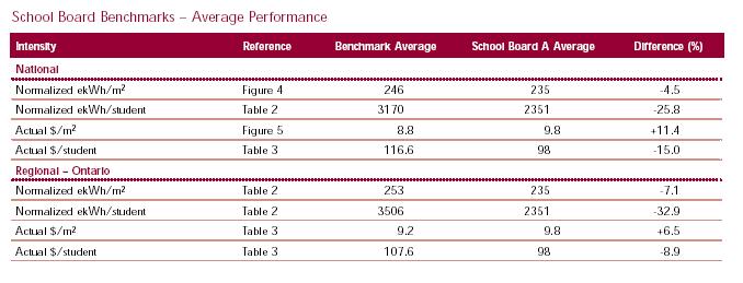
Observations
School Board A's energy intensities - with area as the key impact variable - are lower than the national and Ontario averages. This may suggest that School Board A is more efficient than the national and provincial average school boards. When students are considered, School Board A's intensities are more than 25 percent lower than the national and regional averages.
This may mean that there is a higher density of students in a given location than in other school boards, nationally and regionally. The cost intensity ($/m2) was 11.4 percent higher than the national average, whereas it is relatively the same as the Ontario average. On the other hand, the cost per student intensity is 15 percent lower than the averages.
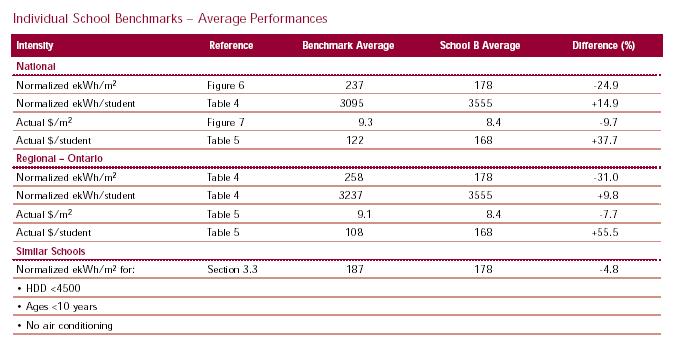
Observations
Secondary School B's energy consumption and cost intensities are significantly lower than the national and regional averages or benchmarks, with differences of about 25 percent. Furthermore, Secondary School B's consumption intensity is 4.8 percent lower than that of other similar schools (i.e. with HDD <4500, age group of less than 10 years, and no air conditioning). It is highly likely that this school is energy efficient and perhaps incorporating "best practices." However, this does not suggest that there are no opportunities for energy efficiency projects at Secondary School B.
Section 5. Calculating Greenhouse Gas (GHG) Emissions
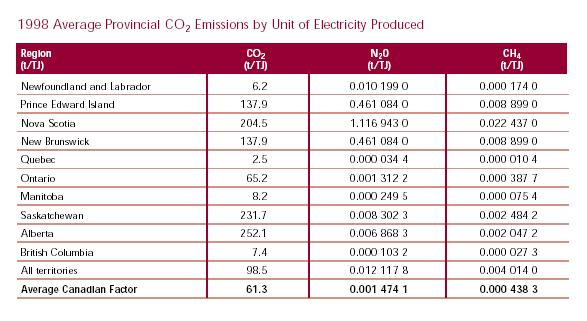
School boards are actively engaged in the national challenge of reducing CO2 emissions. As well, individual sites are registering with Canada's Climate Change Voluntary Challenge and Registry Inc. (VCR Inc.) to record CO2 emissions reductions. Involvement in this national challenge can have strong motivational and educational benefits. Sites wishing to demonstrate commitment to the national targets can convert their benchmark data into equivalent CO2 emissions and see how they relate to the national picture, using appropriate conversion factors.
Standard conversion and emission factors are available from the fuel suppliers or other reference sources, including VCR Inc.'s Registration Guide 1999. Electric utilities that burn a mix of fossil fuels generally provide annual conversion factors for the particular fuel mix used in their generated electricity. School boards' and individual schools' performances can be measured as CO2 emissions through a monitoring and tracking system that uses standard conversion factors for fossil fuels and an annual correction factor for electricity.
To calculate GHG emissions, use the following formulas:
Fossil Fuels:
eCO2 = CO2 + CH4 + N2O
Where,
CO2 = Fuel Consumption 3 EF
CH4 = Fuel Consumption 3 EF for CH4 3 GWP for CH4
N2>O = Fuel Consumption 3 EF for N2O 3 GWP for N2O
Electricity (Indirect Emissions):
eCO2 = CO2 + CH4 + N2O
Where,
CO2 = Electricity Consumption 3 EF
CH4 = Electricity Consumption 3 EF for CH4 3 GWP for CH4 N2O = Electricity Consumption 3 EF for N2O 3 GWP for N2O
And where,
- EF = Emissions Factor for the individual energy source. You can obtain these factors from VCR Inc. or the OEE (see Section 6 for typical values and Section 7 for further references).
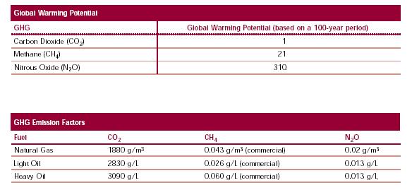
- GWP = Global Warming Potential Factor, the relative global warming potential of different GHGs (compared to CO2). GWP values are available from VCR Inc. As well, typical values are found in Section 6.
Total CO2 Emissions:
eCO2 = eCO2 from Fossil Fuels + eCO2 from Electricity
Tools have been developed to calculate and summarize CO2 emissions. For more information on emissions factors and how you can obtain the tools needed to calculate emissions, see Section 7.
Section 6. Conversion Factors, Energy Contents, GHG Emission Factors and Heating Degree-Days
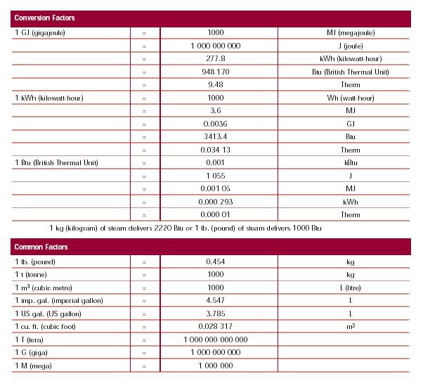

The following is an example of how to convert energy forms.
Question: How much energy will 1000 m3 of gas produce?
i.e. 1000 m3 of natural gas = ? in GJ and ? in kWh
Step 1. Determine the energy content (i.e. how much energy does a cubic metre produce?).
- Look under the Energy Content Factors.
- For natural gas: 1 m3 produces 37.2 MJ or 10.33 ekWh of energy.
Step 2. Calculate the energy content for the amount of natural gas used.
- Energy = 1000 m3 3 37.2 MJ/m3 or 1000 m3 3 10.33 ekWh/m3
- Energy = 37 200 MJ or 10 330 ekWh
Therefore, 1000 m3 of natural gas produces 37 200 MJ or 37.2 GJ or 10 330 kWh of energy.
Sources:
-
Registration Guide 1999, Canada's Climate Change Voluntary Challenge and Registry Inc. (VCR Inc.).
-
Canada's Emissions Outlook: An "Events-Based" Update for 2010,Natural Resources Canada.
-
Demand Policy and Analysis Division, Office of Energy Efficiency, Natural Resources Canada.
Notes:
-
More comprehensive approaches to calculate CO2 emis-
sions are described in the "CO2 Calculations Version 2"
spreadsheet (see Section 7 for references). The spreadsheet includes templates and pre-made formulas to help in the calculations. - There are many ways to determine CO2 emissions resulting from electricity. The factors provided are one of the many methods.
Section 7. Resources
Additional information can be found using the following sources:
Office of Energy Efficiency and Other NRCan Resources
- Best Practices Guide for School Facility Managers
- Benchmarking Guide for School Finance Officers
-
"Dollars to $ense" Workshops:
-The Energy Master Plan
-Energy Monitoring and Tracking
-Spot the Energy Savings Opportunities - Energy Management Action Plan Template and Guidelines
- "CO2 Calculations Version 2" spreadsheet
- Energy Management Series (numerous technical documents ranging from auditing and boilers to energy accounting, compressors and lighting)
- Commercial Building Incentive Program (CBIP) andCommercial Building Incentive Program Technical Guidelines, which refer to the Model National Energy Code for Buildings (MNECB) (see Web site at /cbip)
-
The MNECB and Performance Compliance for Buildings are available from the National Research Council Canada's Institute for Research in Construction (IRC). To order, call
1 800 672-7990 (toll-free) or, in the National Capital Region, call (613) 993-2463.
Fax: (613) 952-7673. - Canada's Emissions Outlook: An Update, Analysis and Modelling Group, National Climate Change Process, 1999.
- The Renewable Energy Deployment Initiative (REDI) (see the Web site at http://www.reed.nrcan.gc.ca/)
These resources, as well as other publications, are all available through the Energy Innovators Initiative of NRCan's OEE at the following:
Energy Innovators InitiativeNatural Resources Canada
Office of Energy Efficiency
580 Booth Street, 18th Floor
Ottawa ON K1A 0E4
Tel.: (613) 995-6950
Fax: (613) 947-4121
Web site:
External Resources and Publications
-
Canadian School Boards Association
Chris Noyes, Project Co-ordinator
Tel.: (613) 235-3724
Fax: (613) 238-0434
E-mail: chris@cdnsba.org
-
Agence de l'efficacité énergétique
Luc Lamontagne, Analyste
Tel.: (418) 627-6379, ext. 8032
Fax: (418) 643-5828
E-mail: luc.lamontagne@aee.gouv.qc.ca
-
Ministère de l'Éducation du Québec
Michel Parent, ing., Direction des équipements scolaires
Direction générale du financement et des équipements
Tel.: (418) 644-2525
Fax: (418) 643-9224
E-mail: michel.parent@meq.gouv.qc.ca
-
Canada's Climate Change Voluntary Challenge
and Registry Inc. (VCR Inc.)
Tel.: (613) 565-5151
Fax: (613) 565-5743
Web site: http://vcr-mvr.ca/
-
ÉcoGESte
Roberte Robert, ing.
Directrice du Programme ÉcoGESte
Bureau d'enregistrement des mesures volontaires sur les changements climatiques
Tel.: (418) 521-3950, ext. 4907
Fax: (418) 646-4320
E-mail: ecogeste@mef.gouv.qc.ca
-
Centre for the Analysis and Dissemination of Demonstrated Energy Technologies (CADDET). This organization is an initiative of the International Energy Agency (IEA).
Michel Lamanque
CADDET Technology Co-ordinator Natural Resources Canada
Tel.: (613) 947-3812
Fax: (613) 947-1016
E-mail: mlamanqu@nrcan.gc.ca
-
ETSU, AEA Technology PLC, Harwell, UK
Tel.: +44 1235 436747
Fax: +44 1235 433066
E-mail: etsuenq@aeat.co.uk
Web site: http://www.energy-efficiency.gov.uk
-
BRECSU, BRE Ltd., Garston, Watford, UK
Tel.: +44 1923 664258
Fax: +44 1923 664787
E-mail: brecsuenq@bre.co.uk
Web site: http://www.energy-efficiency.gov.uk
Buildings Division
Office of Energy Efficiency
Natural Resources Canada
580 Booth Street, 18th floor
Ottawa ON K1A 0E4
Tel.: 877-360-5500 (toll free)
Fax: 613-947-4121
Web site
Page details
- Date modified: