
ARCHIVED - Energy Efficiency in Buildings
Information Archived on the Web
Information identified as archived on the Web is for reference, research or recordkeeping purposes. It has not been altered or updated after the date of archiving. Web pages that are archived on the Web are not subject to the Government of Canada Web Standards. As per the Communications Policy of the Government of Canada, you can request alternate formats. Please "contact us" to request a format other than those available.
Monitoring and Targeting Techniques in Buildings
Background
Monitoring and targeting (M&T) energy use is a critical component of an effective energy management program. M&T techniques provide energy managers and users with feedback on operating practices, results of energy management projects and guidance on the level of energy use that is expected in a certain period.
M&T is a useful tool to not only track energy use but also to control it. It turns data on energy use into useful information that can lead to significant energy and cost savings.
Many industrial organizations use M&T to determine the required energy use for a given set of influencing factors, such as production. They consider energy as a variable cost that fluctuates with the operations, rather than a fixed cost that they have no control over. A similar approach can be taken with energy use in buildings to provide managers with better feedback on how to control their building. In a building, the energy use may vary based on weather (the amount of either heating or cooling required), occupancy, time of year or any other factor that impacts the energy use.
User feedback
Building operators, facility managers and “energy champions” have used M&T to gain insights into their building energy use. Feedback from one school district that uses M&T for 150 energy accounts in 40 buildings provides some interesting insights. Some operators found the information about changes in building energy use helpful and commented, “I like the feedback that you get when you make a change; you can see the impact.” Project managers liked the information on project results and commented, “The graphs made it easy to determine what projects worked well and which ones did not.” The maintenance manager reinforced the benefits as follows: “Previously, we had little idea how much we saved; now we can identify that clearly.” Through many discussions with M&T users, it has become clear that M&T helps turn data into valuable, useable information. In some cases, users have suggested that the data “jumps off the page.”
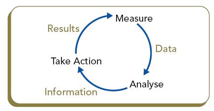
The diagram above illustrates the process applied in M&T, which moves from data to information and ultimately to results. Instead of just taking measurements, the analysis from M&T drives the actions that save energy and costs.
M&T Procedures
The fundamental approach to M&T involves determining what factors will have an influence on energy use, typically recorded by an energy meter. These factors are sometimes referred to as “drivers.” For a building with a natural-gas-fired boiler, the driver will typically be the heating requirements expressed as the number of heating degree-days. For a building with air-conditioning loads and an electric chiller, the driver is often cooling degree-days. The drivers for some building types may also include occupancy.
Once the driving factors are identified, the relationship between the drivers and energy consumption can be established by the technique known as linear regression. Regression analysis attempts to describe the relationship between energy consumption and its drivers with a mathematical equation.
When energy use information is compared with the driver, a regression correlation coefficient, R2, is statistically determined. This is a measure of the proportion of variability explained by the linear relationship in a sample of paired data. It is a number between zero and one, with a value close to zero suggesting a poor model. Generally, a value above 0.7 is considered an acceptable level to have confidence in the relationship; however, a lower value may be acceptable with a larger data set (e.g. two or three years of monthly data).
This regression equation is sometimes referred to as a performance model. The performance model can also be used to predict energy use in a period for a specified set of conditions described by the drivers. Future use can be compared with the prediction to determine whether energy use is higher or lower than predicted. The difference in energy use between actual and target is calculated for each period and added together, creating a “running total.” This is referred to as the CUSUM, or Cumulative Sum, of the differences. The CUSUM is also referred to as the cumulative savings total. Trends in the CUSUM graph indicate consumption patterns. The case studies presented in this fact sheet demonstrate the use of the CUSUM graph. According to one user of M&T, “The CUSUM graph really tells you a story.”
The following examples demonstrate the procedures of M&T in various building types.
Commercial Office Building: Electricity Consumption
The situation
A large multi-storey office complex carried out numerous energy management projects in 2003 and 2004 to improve energy efficiency and modernize the base building systems. In early 2003, an upgrade of the chilled water system was completed, including the installation of two high-efficiency chillers, a new cooling tower, new condenser and chilled water pumps and variable-speed drives. Even though most of the base building lighting had been upgraded in the mid-1990s, late in 2003 a lighting retrofit was undertaken to upgrade the remainder of the building's lighting systems. This retrofit included stairwells, exit signs, storage rooms, incandescent down lights and common area lighting. The final phase of the project was completed in April 2004. It included upgrades to lighting controls to allow nightly lighting “off sweeps” and to heating, ventilating and air-conditioning controls to incorporate current technology. Also, all floor fans were converted from inlet guide vanes to variable-speed-drive operation.
Monitoring
Savings were monitored regularly in 2004 and 2005, and trends were investigated when energy use appeared out of line. Due to the lack of sub-metering data, it would be difficult to determine the energy savings from each of the three projects by using typical savings verification techniques. Additionally, changes in weather needed to be factored into the savings determination. The M&T tool and CUSUM were used to track savings for the separate projects and, more importantly, to ensure that the savings were maintained.
Analysis
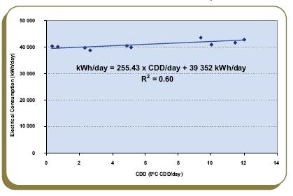
To isolate the impact of building cooling requirements, a regression was carried out on electrical consumption in kilowatt hours (kWh) and cooling degree-days (CDDs), with data from 2002, prior to the retrofits. The best relationship occurred when the building's balance temperature was 6°C. This was rather low compared with those of other buildings, but it was justified due to high internal cooling loads and the lack of free cooling. Even though the R2 was lower than 0.7, it was acceptable because the building's mechanical cooling systems ran 12 months of the year. The relationship between electrical energy use and CDDs is shown in Figure 1. Each point represents the electrical energy use and CDD values for a billing period. The units have been divided by the number of days to eliminate the impact of billing-period length.
FIGURE 1 Electrical versus CDD relationship, 2002
A second regression analysis was carried out to include the initial period, as shown in Figure 1, plus the subsequent two years' post-retrofit, as shown in Figure 2. The second regression analysis does not indicate the varying nature of the relationship over time or when events occurred to change the relationship or performance.
FIGURE 2 Electrical versus CDD relationship, 2002, 2003, 2004

To investigate the changing performance, the baseline or reference period, before the retrofits, was chosen (shown in Figure 1). Savings are measured against that baseline. The CUSUM graph was then constructed using the difference between baseline and actual energy use indicating the sequence of events that improved performance.
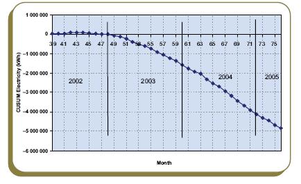
FIGURE 3 Electrical CUSUM, 2002, 2003, 2004, 2005
Interpretation of the CUSUM
Months 39 to 48, on the CUSUM graph in Figure 3, correspond to the same period (2002) shown in the regression in Figure 1. The flat part of the CUSUM line on the left side of the graph indicates that the consumption baseline has no change cumulatively when compared with itself, as would be expected.

This is because we are comparing the period in 2002 with modelled energy use from the same period. When future periods are compared with the baseline, monthly savings are shown, and the slope of the CUSUM line determines the rate of savings. A steeper downward slope represents a greater rate of savings.
Three distinct slopes are evident on the CUSUM graph in Figure 3, representing the three projects carried out. Each change in slope indicates the implementation of a new project and an increase in the rate of savings: the chiller plant savings start in period 48; the lighting retrofit in period 53; and the controls and speed-drive upgrade in period 63. A change in slope is evident at these three points.
CUSUM – Evidence of success
The combined electrical savings for 2003, 2004 and four months of 2005 was 5 million kWh. The annual savings were determined by reading the cumulative value at the end of each year and subtracting it from the previous period. For the last 12-month period, which represents all measures implemented, the savings were 2.5 million kWh, or 20 percent of the baseline annual consumption.
CUSUM – Evidence of success of distinct projects
When multiple projects are in place, the savings from each project can then be isolated from the total savings by following the slope of each line that starts at the beginning of each project's saving period.
Considerable credit needs to go to the building's operating engineers, who worked closely with consultants, contractors and management to optimize the project results. The M&T process was a critical tool used for system optimization.
Health Care Facility: Fuel Consumption
The situation and analysis
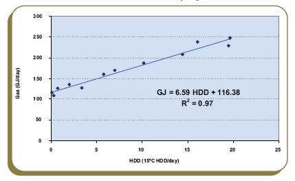
A health care facility manager was interested in determining if M&T could be a useful analysis technique for his energy management program. To decide if the technique would be beneficial, the manager collected and analysed basic data on the main boiler plant's natural gas consumption for three years. The first year was chosen arbitrarily as a baseline or reference period, when gas consumption exhibited a strong dependence on heating degree-days (HDDs). Just over half of the daily gas use was for non-weather-dependent loads, as shown in the regression analysis in Figure 4.
FIGURE 4 Gas versus HDD relationship, year 1
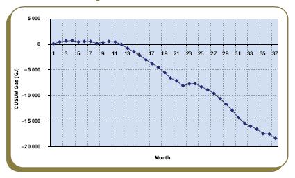
When the CUSUM was plotted for the three years, a significant change became evident. The manager identified from operational records that a heat recovery coil had been installed in the boiler stack to recapture the heat from the flue gases before the gases left the building. As shown in Figure 5, the manager could see the impact and the consistency of the savings, at least initially. An interesting story emerged when the two following years were compared with the base year.
Evidence of success and slippage in savings
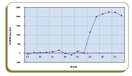
There were considerable energy savings – over 8000 gigajoules (GJ) in the first year (months 13-24) and over 9000 GJ in the second year (months 25-36). However, in two months (months 23 and 24) savings did not occur; in fact, consumption went up slightly. The manager then recalled that during this period, a heat recovery coil had been taken out of service for routine maintenance and had not been immediately reinstalled.
FIGURE 5 Gas CUSUM, years 1, 2 and 3
The manager wondered, "Could this incident have been noticed earlier? And what can I do to ensure that it does not happen again?" One solution is the targeting aspect of M&T. The rate of savings was consistent from months 13 to 22. If this period was chosen as the target consumption, what would indicate a drop in the savings level?
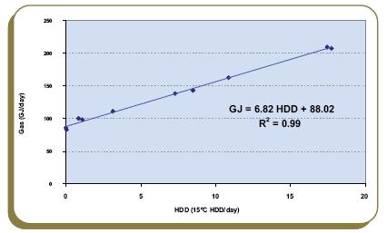
To answer this question, the period from months 13 to 22 was used to determine a target consumption. As with the base period analysis, a regression can be carried out, as shown in Figure 6.
FIGURE 6 Gas versus HDD relationship: target consumption based on improved performance
Based on the new target consumption, a revised CUSUM was prepared. The data for months 23 and 24 say, “Look at me!” Energy use was out of control. The CUSUM graph in Figure 7 shows that the delay in reinstalling the coils "cost" more than 2000 GJ, or nearly $20,000. This highlights the “slippage” in the savings.
FIGURE 7 Gas CUSUM: shows impact of operational change in month 23
Targeting as a means of control
Using a control chart, similar to control charts used in quality assurance programs, can expand the concept of the target. The control chart sets upper and lower limits of acceptable operations. The upper limit flags performance operations that are not meeting the target. The lower limit indicates even better performance – perhaps this performance could be investigated to determine if the operation could continue in this manner. If that was the case, then a new target could be set.
The control chart in Figure 8 shows the difference each month between actual and predicted use. Months 23 and 24 are out of control. Month 31 would be a good month to ask, “What did we do well?”
FIGURE 8 Control chart used to target gas consumption
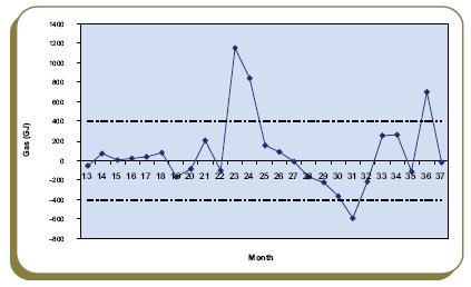
Developing a control chart would allow this facility manager to catch and correct poor energy performance and to capture and replicate periods of best energy performance.
Elementary School: Fuel and Electricity Consumption
The situation
A school district used M&T to review a series of energy projects that had been carried out. Previously, it knew that it was achieving energy savings through an in-house program of lighting and controls upgrades. However, it did not know the extent of the savings. A number of CUSUM graphs provide insights into the applications of M&T.
CUSUM – Evidence of seasonal savings
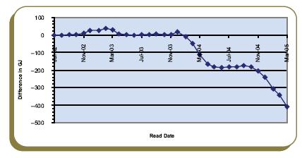
In one of the smaller elementary schools, natural gas use was reviewed after night set-back was implemented in the school. This established a strong relationship (correlation coefficient of 98 percent) between natural gas and HDDs. In Figure 9, the CUSUM shows annual savings of almost 200 GJ each year, with the savings occurring in the winter months. The savings are minimal during the summer months, as shown by the flat section of the CUSUM graph in 2004. The rate of savings in the winter months is consistent in the two years' post-implementation.
FIGURE 9 Gas CUSUM showing savings in winter 2003/04 and 2004/05 D

CUSUM – Evidence of savings from multiple actions
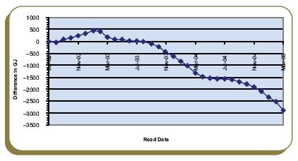
In one of the larger secondary schools, natural gas use was also reviewed and compared with HDDs. In Figure 10, the CUSUM shows annual savings of almost 1600 GJ each year, again with the savings occurring in the winter months. In this case, the boiler had been replaced with a more efficient unit, and the building automation system had been reprogrammed. While individual savings cannot be identified, we can state with confidence that the overall savings were 1500 GJ/year, or about 30 percent. Note that the CUSUM analysis, and the savings that you can see in the chart, adjust for the impact of a mild or severe winter on your savings calculation. Savings are based on “what you would have used” given the weather conditions that occurred.
FIGURE 10 Gas CUSUM with total savings of almost 3000 GJ
CUSUM – Evidence of consistent savings
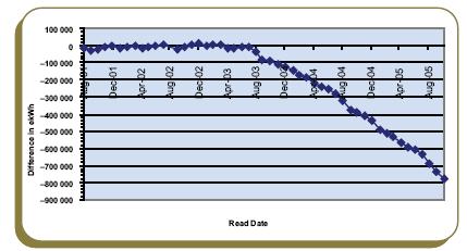
In another larger secondary school, electricity use was reviewed. It was determined that HDDs was the driver, since the buildings also used electric heating. In Figure 11, the CUSUM shows annual savings of over 230 000 kWh each year. In this case, the CUSUM shows the impact of a lighting retrofit in 2003. The good news was the level of consistency of the energy savings, which was over 20 percent annually.
FIGURE 11 Electrical CUSUM with consistent savings rate
CUSUM – a tool to investigate elevated consumption
The school district also used the CUSUM analysis to identify accounts where energy use was higher than expected. In one school, an increase in energy use was attributed to a building operator's manual overrides. In another case, the CUSUM showed the increase in natural gas use could be attributed to the school's recent ventilation upgrade. By plotting a CUSUM graph for historical consumption, it is possible to identify when changes occurred and to correlate these changes to physical events in the facility.
Summary
These examples show that M&T can be applied in the building sector to help manage energy use, detect changes and problems in operations, and calculate savings from projects and improved operational techniques. M&T is a worthwhile addition to any energy monitoring program, getting people into the energy information feedback loop.
We can only manage what we measure. And we can manage well with M&T techniques!
Buildings Division
Office of Energy Efficiency
Natural Resources Canada
580 Booth St., 18th floor
Ottawa ON K1A 0E4
Tel.: 877-360-5500 toll free
Fax: 613-947-4121
Web site
Page details
- Date modified: